Obtaining Data
A single simulation gives you one timecourse. To make a dataset, you need to vary the model — perturb initial conditions, perturb kinetic parameters, or both — and simulate each variation. That's what make_dataset_drug_response does.
This page covers the shape of the resulting dataset, the perturbation strategies, and how to control what's exposed per sample.
The Basic Call
from synthetic import Builder, make_dataset_drug_response

vc = Builder.specify(degree_cascades=[3, 6, 15], random_seed=42)

X, y = make_dataset_drug_response(
    n=1000,
    cell_model=vc,
    target_specie='Oa',
)

print(f"Features: {X.shape}")  # (1000, n_features)  — one column per species
print(f"Target:   {y.shape}")  # (1000,)             — one value per simulation
Xis apandas.DataFrame. Each column is a species name (R1_1,I1_1,Oa, ...). Each row is one simulation.yis apandas.Series. The value is the concentration of the target species at the end of the simulation.- The two are aligned: row
iofXand elementiofycame from the same perturbed run.
The result drops into any scikit-learn workflow unchanged.
Levels of Data per Sample
make_dataset_drug_response exposes a spectrum of information per simulation. You choose how much to take.
| Level | Flag | What you get per sample |
|---|---|---|
| 0 (default) | none | Initial-condition features (one per species) and the final value of the target species |
| 1 | return_timecourse=True |
+ full numpy-array timecourse for every species |
| 2 | (no flag — comes with level 1) | + DataFrame of kinetic parameters (Km_J0, Vmax_J1, ...) |
| 3 | (derived in user code) | Last-point features of the activated species, or any other timecourse-derived representation |
Level 0 is enough for most regression use cases. Level 1 unlocks the full simulation history — useful for parameter estimation (you can mimic sparse experimental observations), timecourse feature engineering, and validation. Level 3 is what ML papers actually compare when they ask "which feature representation predicts drug response best?" — see Use Cases.
What Gets Perturbed
By default, each sample uses a conservation-rules perturbation: the total concentration of each species pair (e.g., R1_1 + R1_1a) is held constant, but the ratio between the inactive and active forms is varied. This produces biologically plausible initial conditions — you never get "all zero" or "all active" start states.
To use a different distribution:
# Gaussian perturbation of initial conditions
X, y = make_dataset_drug_response(
    n=100, cell_model=vc,
    perturbation_type='gaussian',
    perturbation_params={'rsd': 0.2},  # 20% relative standard deviation
)

# Lognormal perturbation
X, y = make_dataset_drug_response(
    n=100, cell_model=vc,
    perturbation_type='lognormal',
    perturbation_params={'rsd': 0.2},
)

# Latin Hypercube Sampling — better space-filling
X, y = make_dataset_drug_response(
    n=100, cell_model=vc,
    perturbation_type='lhs',
    perturbation_params={'rsd': 0.2},
)
| Type | Distribution | Parameters |
|---|---|---|
conserve_rules |
Conservation-law ratio (default) | shape, base_shape, max_shape |
uniform |
Uniform | min, max |
gaussian |
Normal | rsd |
lognormal |
Log-normal | rsd |
lhs |
Latin Hypercube | rsd |
Perturbing Kinetic Parameters Too
The initial conditions are one source of variation. The kinetic parameters (Km, Vmax, ...) are another, and they're often more predictive of drug response than initial concentrations. You can perturb both:
X, y = make_dataset_drug_response(
    n=100, cell_model=vc,
    perturbation_type='gaussian',                     # for initial conditions
    perturbation_params={'rsd': 0.2},
    param_perturbation_type='lognormal',              # for kinetic parameters
    param_perturbation_params={'shape': 0.1},
    param_seed=42,                                    # separate seed from initial-cond perturbations
)
Reproducibility
Two seeds control reproducibility:
random_seedonBuilder.specify(...)— fixes the network topology and the drug configuration.seed(andparam_seed) onmake_dataset_drug_response(...)— fixes the perturbations applied to generate samples.
Use both for fully reproducible datasets:
vc = Builder.specify(degree_cascades=[3, 6, 15], random_seed=42)
X, y = make_dataset_drug_response(
    n=1000, cell_model=vc,
    seed=42,         # initial-condition perturbations
    param_seed=42,   # kinetic-parameter perturbations
)
Extended Return Format
For ML research, you usually want more than (X, y) — you want the full timecourse and the kinetic parameters that produced each sample. Use return_timecourse=True:
result = make_dataset_drug_response(
    n=500, cell_model=vc, target_specie='Oa',
    return_timecourse=True,
)

X            = result['X']            # feature matrix (initial conditions)
y            = result['y']            # target vector
timecourse   = result['timecourse']  # DataFrame of numpy arrays — one row per sample
parameters   = result['parameters']  # DataFrame of kinetic parameters per sample
metadata     = result['metadata']    # success rate, simulation range, etc.

print(f"Success rate: {metadata['success_rate']:.2%}")
The timecourse rows contain numpy arrays — one array per species, holding the concentration at each simulation timepoint. To extract, e.g., the last timepoint of each species per sample:
import numpy as np
import pandas as pd

last_point_features = []
for _, sample_tc in timecourse.iterrows():
    last_point_features.append({
        col: arr[-1] for col, arr in sample_tc.items() if arr is not None
    })
X_last = pd.DataFrame(last_point_features)
See Use Cases for end-to-end examples that consume this format — parameter estimation, classification, and ML model comparison.
Controlling the Simulation
X, y = make_dataset_drug_response(
    n=100, cell_model=vc,
    simulation_params={'start': 0, 'end': 8000, 'points': 101},
)
start— simulation start timeend— simulation end time (default uses the model'ssimulation_end, typically 10000)points— number of timepoints to record
Solver Choice
By default, make_dataset_drug_response uses ScipySolver with jit=True. For other options:
# ScipySolver (default, fast with JIT)
X, y = make_dataset_drug_response(n=100, cell_model=vc, solver_type='scipy', jit=True)

# RoadrunnerSolver (robust, full SBML)
X, y = make_dataset_drug_response(n=100, cell_model=vc, solver_type='roadrunner')

# HTTPSolver (remote)
X, y = make_dataset_drug_response(n=100, cell_model=vc, solver_type='http',
                                  solver_endpoint='http://localhost:8000/simulate')
See Solving ODEs for the comparison, JIT warmup cost, and the trade-offs between solvers.
Feature Analysis: Which Species Matter?
In a hierarchical network, the degree 1 species (closest to the drug) usually correlate most strongly with the outcome. To check:
Top-left: feature correlation matrix. Top-right: feature-target correlation. Bottom: outcome distribution.
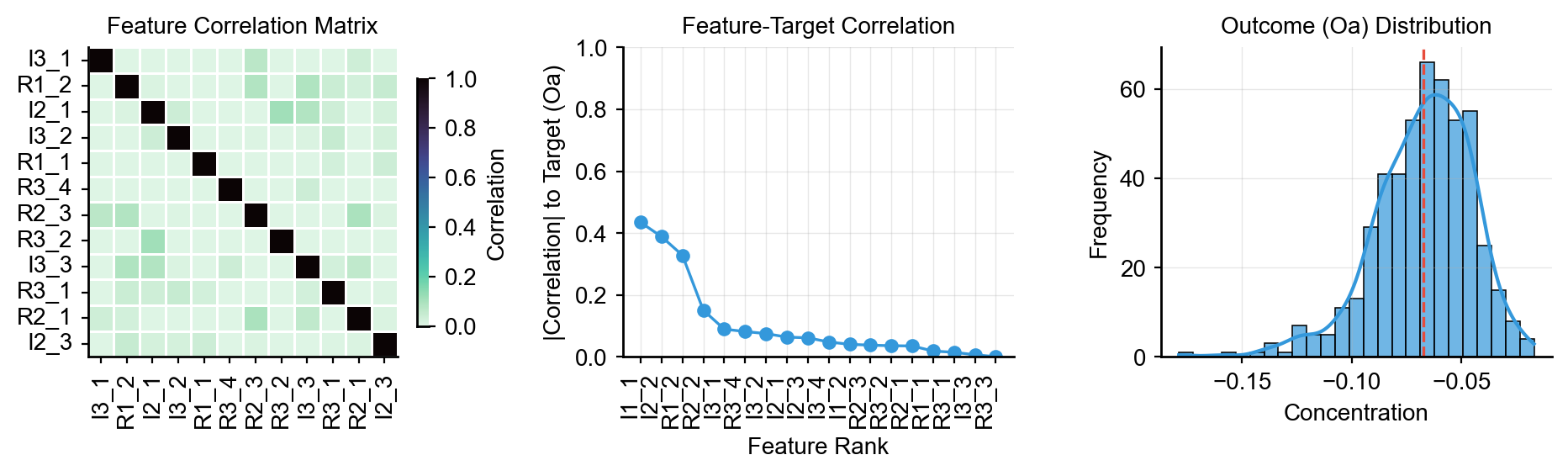
correlations = X.apply(lambda col: col.corr(y))
correlations = correlations.reindex(correlations.abs().sort_values(ascending=False).index)
print("Top 10 features correlated with target:")
print(correlations.head(10))
For more sophisticated feature analysis — feature engineering from the full timecourse, comparing ML models across feature representations — see Use Cases.
Exporting Data
X.to_csv('synthetic_features.csv', index=False)
y.to_csv('synthetic_targets.csv', index=False, header=['target'])
combined = pd.concat([X, y], axis=1)
combined.to_csv('synthetic_dataset.csv', index=False)
Next: Use Cases — finished end-to-end examples that consume the dataset.