Solving ODEs
Once you have a model, the next step is running it: integrate the ODE system forward in time and capture the species concentrations. That's what a solver does. The output of a solver is a timecourse — a pandas.DataFrame with a time column and one column per species.
If you're building a dataset rather than studying one simulation, see Obtaining Data — that page uses solvers internally and packages the output as scikit-learn-shaped (X, y).
What a Solver Does
A solver takes a model (Antimony or SBML), an initial state, and a time range, and returns the species concentrations at each time point. Synthetic ships three solvers:
| Solver | Input | Strengths |
|---|---|---|
ScipySolver |
Antimony | Fast, Numba JIT for batch work, default choice |
RoadrunnerSolver |
SBML | Robust, full SBML feature support. Accepts any SBML — including ones not produced by Synthetic. |
HTTPSolver |
HTTP endpoint | Remote simulation across machines |
All three return a pandas.DataFrame with a time column and one column per species:
       time    R1_1   R1_1a    I1_1   I1_1a      O      Oa
0       0.0  100.00    0.00  100.00    0.00  100.0    0.0
1      50.0   95.23    4.77   98.10    1.90   99.5    0.5
2     100.0   91.50    8.50   96.40    3.60   98.8    1.2
...
The Easy Path: make_dataset_drug_response
You don't usually need to touch a solver directly. The high-level make_dataset_drug_response function picks one for you, runs it many times with perturbations, and returns the dataset:
from synthetic import Builder, make_dataset_drug_response

vc = Builder.specify(degree_cascades=[3, 5], random_seed=42)

# ScipySolver (default) — fast, JIT-compiled
X, y = make_dataset_drug_response(n=100, cell_model=vc, solver_type='scipy', jit=True)

# RoadrunnerSolver — robust, requires the [roadrunner] extra
X, y = make_dataset_drug_response(n=100, cell_model=vc, solver_type='roadrunner')

# HTTPSolver — remote simulation
X, y = make_dataset_drug_response(n=100, cell_model=vc, solver_type='http',
                                  solver_endpoint='http://localhost:8000/simulate')
See Obtaining Data for the full API — return formats, perturbation strategies, parameter sweeps.
Direct Solver Usage
When you want a single timecourse (one simulation, not a dataset), use a solver directly.
ScipySolver
Uses scipy.integrate.odeint with optional JIT compilation:
from synthetic.Solver.ScipySolver import ScipySolver

vc = Builder.specify(degree_cascades=[2, 3, 4], random_seed=42)
antimony = vc.model.get_antimony_model()

solver = ScipySolver()
solver.compile(antimony, jit=True)              # compile once
results = solver.simulate(start=0, stop=10000, step=50)
print(results.head())
The compile step is slow on first call (JIT warms up); subsequent simulations on the same compiled model are fast. This is a one-time cost per model.
RoadrunnerSolver
Uses libRoadRunner for SBML simulation:
from synthetic.Solver.RoadrunnerSolver import RoadrunnerSolver

sbml = vc.model.get_sbml_model()
solver = RoadrunnerSolver()
solver.compile(sbml)                            # note: SBML, not Antimony
results = solver.simulate(start=0, stop=10000, step=50)
Requires SBML format
RoadrunnerSolver.compile(...) requires an SBML string (or path). Use vc.model.get_sbml_model(), not get_antimony_model().
Using External SBML
RoadrunnerSolver is not limited to Synthetic-built models — it consumes any SBML:
# Load an SBML file produced by COPASI, Antimony, BioNetGen, etc.
solver = RoadrunnerSolver()
solver.compile('path/to/external_model.sbml')
results = solver.simulate(start=0, stop=1000, step=10)
This makes RoadrunnerSolver a useful entry point into the Synthetic ecosystem for users who already have SBML models from elsewhere.
HTTPSolver
Sends simulation requests to a remote server. Useful for distributed computing or when the simulation engine runs on a separate machine:
from synthetic.Solver.HTTPSolver import HTTPSolver

solver = HTTPSolver()

# Connect and validate endpoint
solver.compile("http://localhost:8000/simulate")

# Get default states and parameters
states = solver.get_state_defaults()
params = solver.get_parameter_defaults()

# Override values
solver.set_state_values({"R1_1": 1000.0})
solver.set_parameter_values({"Km_J0": 10.0})

# Run simulation
results = solver.simulate(start=0, stop=60, step=0.5)
The server side of the contract is in examples/httpsolver_api.md, with a working FastAPI example. For writing your own server-side implementation, see Advanced.
Choosing a Solver
| Scenario | Recommended |
|---|---|
| Default dataset generation | ScipySolver, jit=True |
| Batch simulations (1000+ samples) | ScipySolver, jit=True (one-time warmup pays off) |
| A single, complex SBML model | RoadrunnerSolver |
| Loading an SBML file from outside Synthetic | RoadrunnerSolver |
| Parameter estimation loop (many short sims) | ScipySolver, jit=False (avoid recompile) |
| Distributed / remote simulation | HTTPSolver |
Verifying Both Solvers Agree
If you're using RoadrunnerSolver because you need its robustness, sanity-check that it gives the same trajectory as ScipySolver for a simple model:
from synthetic.Solver.ScipySolver import ScipySolver
from synthetic.Solver.RoadrunnerSolver import RoadrunnerSolver

solver_scipy = ScipySolver()
solver_scipy.compile(vc.model.get_antimony_model(), jit=False)
tc_scipy = solver_scipy.simulate(start=0, stop=10000, step=50)

solver_rr = RoadrunnerSolver()
solver_rr.compile(vc.model.get_sbml_model())
tc_rr = solver_rr.simulate(start=0, stop=10000, step=50)

print(f"ScipySolver Oa at t=10000: {tc_scipy['Oa'].iloc[-1]:.4f}")
print(f"RoadrunnerSolver Oa at t=10000: {tc_rr['Oa'].iloc[-1]:.4f}")
# Should match to within solver tolerance
Plotting a Timecourse
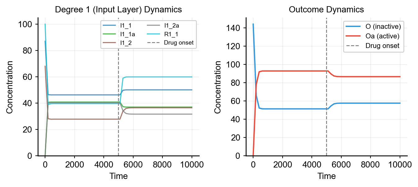
The most common reason to use a solver directly: see what the drug does to the outcome.
import matplotlib.pyplot as plt

vc = Builder.specify(degree_cascades=[2, 3, 4], random_seed=42)
antimony = vc.model.get_antimony_model()

solver = ScipySolver()
solver.compile(antimony, jit=False)
tc = solver.simulate(start=0, stop=10000, step=50)

fig, ax = plt.subplots()
ax.plot(tc['time'], tc['O'], label='O (inactive outcome)')
ax.plot(tc['time'], tc['Oa'], label='Oa (active outcome)')
ax.axvline(5000, color='gray', linestyle='--', label='Drug onset')
ax.set_xlabel('Time')
ax.set_ylabel('Concentration')
ax.legend()
plt.show()
The vertical dashed line is when the auto-drug activates. The outcome Oa typically rises or falls in response.
Timecourse produced by ScipySolver. Dashed line marks drug onset.
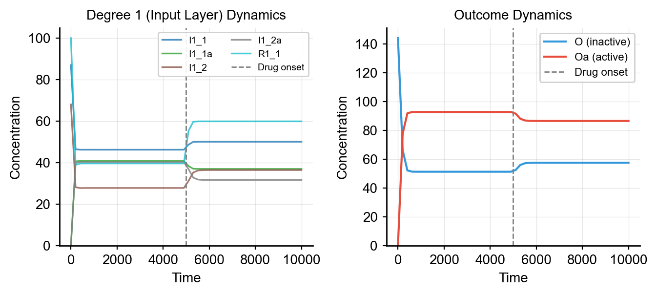
The same model run with RoadrunnerSolver — identical dynamics:
Timecourse produced by RoadrunnerSolver — identical dynamics to ScipySolver.
Next: Obtaining Data — once you can produce one timecourse, the next step is producing many, packaged as a dataset.